Use of Phylogenetic Analysis to Study Evolutionary Relationships

I. Objectives:

1. To learn how to do phylogenetic analysis as a means of analyzing and predicting evolutionary relationships

II. Background:

The evolution of living organisms has two components. The first is the vertical or timewise component, which gives rise to different “grades” of specialization (ancestral vs. advanced traits). However, if that was the only component, there would only be one species that would become increasingly more advanced, only exhibiting directional change through time. The second, the horizontal, component is diversification, the degree of divergence into different lines or “clades” (clado = branch, sprout) that has taken place from the ancestral condition to the present diversity of forms.

Phylogeny is the study of the evolutionary development or history of a group of organisms (phylo = tribe). Classic phylogeny looks at and compares individual species, while other branches of phylogeny expand upon that, looking at larger groupings of organisms such as genera, families, orders, etc., which, then, are often referred to as “operational taxonomic units” or “OTUs.”

While there are exceptions to the rule, in general, organisms with similar structures have a common evolutionary lineage. Thus we observe, for example, that there are quite a variety of organisms around us which are covered in feathers and have their front limbs modified as wings. Biologists believe that those similarities in appearance, are an indication that those organisms are all related, a grouping which we call “birds.”

However, at times, the presence of certain traits may not accurately indicate evolutionary relationships. For example, a fish is aquatic, and that is considered a “primative” or “ancestral” condition, yet the aquatic lifestyle of whales is considered an advanced trait because they are “secondarily aquatic,” having evolved from terrestrial ancestors. Thus, the traits used in the comparison of organisms must be carefully chosen. The outcome of the phylogenetic analysis, the predicted evolutionary relationships, is/are only as good as the validity of the traits one has used to compare the organisms involved.

Biologists also believe that the stages in, the progression of, the embryonic development of a species goes through a series of stages analogous to all the steps in the evolutionary history of that species, summed up by the phrase, “ontogeny recapitulates phylogeny” (onto = being, existing; phylo = tribe; -geny = production), and thus, comparative embryology is also used in the determination of evolutionary relationships.

In performing a phylogenetic analysis, first the specimens and/or taxonomic groups to be compared are identified. Often, 10 to 20 individuals or groups are compared. Using fewer taxa might result in a skewed, inaccurate analysis, and using considerably more taxa could result in difficulty determining valid traits to use and/or unwieldy calculations.

Then, the most significant traits are identified and quantified. For each trait, a “primitive” or “ancestral” form is identified and assigned a value of “0” and an “advanced” form is identified and assigned a value of “1.” As an example, when comparing various animals, the method of providing nutrients to the embryos is one trait that might be included. In that case, embryonic development within an egg which may include a yolk and be surrounded by an eggshell would be considered a primitive trait and be assigned a value of “0,” while embryonic development within the mother’s uterus, attached to a placenta via an umbilical cord, would be considered an advanced trait and be assigned a value of “1.” These need to be either/or, yes/no choices, so for example, if the number of toes an animal has is one of the traits that would be useful, that could not be broken down into categories of 5 toes vs 4 toes vs 2 toes vs 1 toe, but rather, would need to be divided into something such as full number of toes (5) as the primitive trait, and reduced number (2-toed and 1-toed grouped together) as the advanced trait. Again, this would only work if those groupings are legitimate, accurate categories to use for the group of organisms being compared: for example, domestic dogs usually only have four toes. While enough traits must be provided to reliably distinguish evolutionary relationships, there is also an upper limit to the useful number of traits, above which no more information will be gained. Thus, it is common to use between 60 and 100 traits when doing this type of analysis.

Next, a table/matrix is created in which each taxon is assigned a value of “0” or “1” for each of the traits being used. Following creation of that data matrix, a number of calculations are performed, and the resulting data are graphed to show the evolutionary relationships. The resulting phylogenetic trees can only show which split occurred 1^st, 2^nd, etc., but in and of themselves, tell nothing about the timing of those splits (that would have to be determined by other means). Also, divergence (the list of taxa being compared) is typically shown in equal units across the width of the paper.

III. Materials Needed:

• calculator
• semicircular graph paper (attached)
• protractor

IV. Procedure:

For this lab, work in groups of 4 to 5 people so you can share and discuss ideas as you work through the following steps.

1. Determine the taxa which will be compared. As an example of how to do the calculations, the farm animals mentioned in the Taxonomy Lab (duck, chicken, pig, cow, and horse) will be used, with the addition of a lizard. For this lab, you are asked to compare the orders of insects listed in the Data section, below.
2. Determine the traits which will be used to compare those taxa, and for each trait, designate a “primitive” and “advanced” form. For example, for the farm animals, I came up with these ten traits:
   1. Body Covering:
      (0) scales or modified scales (feathers)
      (1) hair
   2. Number of Toes:
      (0) 4 or 5
      (1) 1 or 2
   3. Webbing between toes
      (0) absent
      (1) present
   4. Embryonic Development
      (0) eggs in egg shell (oviparous)
      (1) young in uterus with placenta (viviparous)
   5. Digestion
      (0) food continues through system
      (1) specialized 4-part stomach with fermentation & regurgitation
   6. Body Temperature Regulation
      (0) cold-blooded
      (1) warm blooded
   7. Large Canine Teeth/Tusks
      (0) absent
      (1) present
   8. Heart, Num. of Chambers
      (0) 3-chambered
      (1) 4-chambered
   9. Type of Front Limbs
      (0) front limbs modified for walking
      (1) front limbs modified for flying
   10. Presence of Horns on Head
       (0) none
       (1) horns present
   For the insect orders that you are to use, because coming up with a valid set of traits to use can be a bit difficult, it is suggested that you use the traits listed below for your analysis.
3. Create a table to assign values to each taxon for each trait. The traits are listed across the top, and the taxa are listed down the side. An additional column is added to calculate a total for each taxon. For the farm animals in the example, this table would look like this.
   

   	body	toes	web	eggs	rumen	temp	teeth	heart	arms	horns	Σ=
   lizard	0	0	0	0	0	0	0	0	0	0	0
   duck	0	0	1	0	0	1	0	1	1	0	4
   chicken	0	0	0	0	0	1	0	1	1	0	3
   pig	1	1	0	1	0	1	1	1	0	0	6
   cow	1	1	0	1	1	1	0	1	0	1	7
   horse	1	1	0	1	0	1	0	1	0	0	5

   Table 1. Data Matrix for Farm Animals
   In the Data section, below, a similar table has been created for the insect orders you are to analyze. Each taxon has been ranked for each trait by assigning a value of “0” or “1” as appropriate. (If you are not sure how to rank a particular trait for a particular taxon, you are encouraged to use a book or a computer to find the necessary information.)
4. Create a matrix table to count the number of traits each taxon has in common with each other taxon. Each taxon is listed both across the top and down the side. The number of traits in common with each other taxon is listed in the appropriate box. For the farm animals, this would look like this:

   	lizard	duck	chicken	pig	cow	horse
   lizard	—	6	7	4	3	5
   duck		—	9	4	3	5
   chicken			—	5	4	6
   pig				—	7	9
   cow					—	8
   horse						—

   In your lab notebook, create a similar table to determine how many of the traits the insect orders have in common with each other. Note that if both taxa have a “1” that is a match, and if both taxa have a “0” that also is a match.
5. Perform a “cluster analysis.” For the first step in this process, all you need to do is figure what fraction of the total number of traits each of the numbers, above, represents. Thus, for example, if as shown above, the lizard and duck share 6 traits in common out of a total of 10 traits being used in this example, then 6/10 = 0.60. For the farm animals, this would look like this (note that the pairs which are highlighted share the highest number of traits in common with each other):

   	lizard	duck	chicken	pig	cow	horse
   lizard	—	6/10=0.60	7/10=0.70	4/10=0.40	3/10=0.30	5/10=0.50
   duck		—	9/10=0.90	4/10=0.40	3/10=0.30	5/10=0.50
   chicken			—	5/10=0.50	4/10=0.40	6/10=0.60
   pig				—	7/10=0.70	9/10=0.90
   cow					—	8/10=0.80
   horse						—

   In your lab notebook, create a similar table for the insect orders, remembering that you are dealing with a total of 30 traits. Note, in the example, above, the pair of taxa (in this case two pairs of taxa were “tied”) with the highest percentage in common were highlighted because that/those pairs will be used in the next step. That/those highest percentage(s) is/are an indication that those two taxa have the most traits in common, and thus presumably, are the most closely related.
6. Combine the most closely-related pair(s) and re-compare all the taxa by calculating averages where needed. For example, in the table, above, the relationship between lizard and cow would not change. However, to re-calculate the relationship between lizard and the duck-chicken combination, since lizard and duck have 0.60 in common and lizard and chicken have 0.70 in common, those two numbers would be averaged, so (0.60 + 0.70)/2 = 0.65. Thus, for the farm animals, the combined numbers would look like this:

   	lizard	duck-chicken	pig-horse	cow
   lizard	—	(0.60+0.70)/2=0.65	(0.40+0.50)/2=0.45	0.30
   duck-chicken		—	(0.4+0.5+0.5+0.6)/4 =0.50	(0.30+0.4)/2=0.35
   pig-horse			—	(0.70+0.80)/2=0.75
   cow				—

   In your lab notebook, create a similar table for the insect orders. Note, in the example, above, once again, the pair with the highest percentage in common were highlighted because that pair will, once again, be combined in the next step.
7. Continue to combine the most closely-related pair(s) and re-compare all the taxa. Continue this process until all taxa have been combined. For the farm animals, the following steps would be needed:
   As shown in the previous table, the combination of pig-horse with cow has the next-highest percentage, so that would be combined next.

   	lizard	duck-chicken	pig-horse-cow
   lizard	—	0.65	(0.45+0.30)/2 =0.38
   duck-chicken		—	(0.50+0.35)/2 =0.42
   pig-horse-cow			—

   Similarly, lizard with duck-chicken is next highest, so would be combined next.

   	lizard-duck-chicken	pig-horse-cow
   lizard-duck-chicken	—	(0.38+0.42)/2 =0.40
   pig-horse-cow		—

   In your lab notebook, do these calculations for the insect orders.
8. While all data needed for the next step are present in the tables you have just created, it can be useful, at this point, to make a list of the “important” data, just because it’s easier to see at a glance. Thus, for the farm animals:
   • chicken+duck and pig+horse are both at 0.90
   • pig-horse+cow is at 0.75
   • lizard+duck-chicken is at 0.65
   • the two branches come together at 0.40
9. Create a dendrogram. This is a graph of the data which indicates where the various taxa split from each other. The taxa should be listed, equally-spaced, across the top of the page/graph, but thought is needed, first, to determine the order in which they should be listed. For example, for the farm animals, if they are listed in the order, “lizard, duck, chicken, pig, cow, horse” that will cause a problem because pig and horse are one of the first pairs to be combined, and thus, must be listed next to each other.
   The Y-axis represents the percentage of shared traits. If you start your graph at the top of your lab notebook page, right under your cross references and let each space represent 0.02 units, the bottom of the graph won’t go all the way down to zero at the bottom of the page, but should be low-enough to include all the data.
   
   Farm Animal Dendrogram For the taxa which are the most closely related, draw a line down from each of those taxa to the level where they are related, and at that level, join them with a horizontal line. For example, for our farm animals, a line would be drawn down from chicken and duck to the 0.90 level, at which point a horizontal line would connect those lines. A line would be drawn from the center of that connector down to the next level, and there, connected with the appropriate taxon. For the farm animals, the dendrogram would look like this. (Note that to save space, on the graph, “Lz” = lizard, “Ch” = chicken, “Dk” = duck, “Pg” = pig, “Hr” = horse, and “Cw” = cow.)
   
   Use the numbers you have calculated for the insect orders to draw a dendrogram for that group of organisms.


Semicircular Graph Paper

10. Create a semicircular graph. This is an alternative way to represent the same data. Use the semicircular graph paper (above) which is included with this protocol (this was turned sideways because it fit better that way).
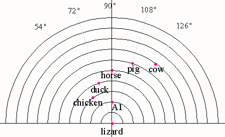
    Find the taxon with the lowest total index score (so that’s presumably the least advanced one). This is considered the most primitive taxon and serves as the standard of comparison for the others.
    Place a dot for that taxon on the baseline of the graph, to the left of center. The distance to the left is its total index score values, which is its degree of evolutionary advancement.
    Again, continuing the farm animals example, first, examine the right-hand column of Table 1 (above), and look for the taxon with the lowest total (thus, the most primitive). In the case of the farm animals, that would be the lizard, which has a total of 0 advanced traits (that’s a bit unusual, and only a result of the traits that were chosen — usually the lowest taxon has a total greater than zero). Go out that many units straight to the left of (0,0), along the x-axis, and put a dot there to represent that taxon.
    For each subsequent taxon, the distance out from the center represents the degree of evolutionary advancement and the “angle of radius with the baseline” represents the degree of divergence from the standard of comparison.
    Thus, for each of the other taxa, two numbers will be needed: that taxon’s total, as well as how many traits (no matter whether a “0” or a “1”) that taxon shares in common with the most primitive one, identified above (symbolized by “r”). It might help to summarize these numbers in another table. For the farm animals being used as an example, this would look like:
    

    	Σ =	# in common w/ lizard
    chicken	Σ=3	r=7
    duck	Σ=4	r=6
    horse	Σ=5	r=5
    pig	Σ=6	r=4
    cow	Σ=7	r=3

    Next, the divergence, the angle up from the left side of the X-axis, symbolized by “D,” must be calculated for each taxon. If the total number of characters being compared is symbolized by “x” (for the farm animals, 10 traits are being compared), the formula for D is
    

    D = (x–r) ×	(	180°	)
    		x

    Thus, for the farm animals:
    

    	Σ =	D =
    chicken	Σ=3	D=(10–7)×18=54°
    duck	Σ=4	D=(10–6)×18=72°
    horse	Σ=5	D=(10–5)×18=90°
    pig	Σ=6	D=(10–4)×18=108°
    cow	Σ=7	D=(10–3)×18=126°

    Each taxon will be plotted on the semicircular graph “Σ” units/rings out from the center and “D” degrees up from the left side of the X-axis. For example, because chicken has a total score of 3, it gets plotted on the “3” circle, 54 up from the left side of the X-axis.
    Then, a common ancestor for all but the most primitive taxon must be calculated. Excluding the taxon that was chosen as the most primitive (lizard), next determine a common ancestor (A1) for the remaining taxa. First, find all the characters-in-common that all of them share. The sum of scores for the positive matches equals the total index score for the common ancestor A1. For example:
    

    	body	toes	web	eggs	rumen	temp	teeth	heart	arms	horns	Σ=
    lizard	0	0	0	0	0	0	0	0	0	0	0
    duck	0	0	1	0	0	1	0	1	1	0	4
    chicken	0	0	0	0	0	1	0	1	1	0	3
    pig	1	1	0	1	0	1	1	1	0	0	6
    cow	1	1	0	1	1	1	0	1	0	1	7
    horse	1	1	0	1	0	1	0	1	0	0	5
    A1	—	—	—	—	—	1	—	1	—	—	2

    To determine the radius on which common ancestor A1 lies, calculate the mean of the divergence values for all the taxa except the first one, so
    

    DA1 =	Σ Dtaxa
    	N

    In other words, average the degrees, so for chicken, duck, horse, pig, and cow, D_A1=(54+72+90+108+126)/5=90. That means that, for the farm animals, A1 would be on the 2 circle, 90 up. Thus, for the farm animals, so far the graph would look like the Partial Graph, below.
    Next, any other needed common ancestors would be calculated in a similar manner. By visual inspection, look for what looks like clusters of taxa. For each cluster, find a common ancestor (A2, A3, etc.) by averaging all the values for the taxa in that cluster. If A2 has the same index score as A1, that means the cluster is artificial and one or more of its taxa don’t belong in the cluster, but come separately off A1.
    Again using the farm animals as an example, after plotting the various points as calculated, above (and from looking at the Partial Graph), chicken and duck look “clumped,” and the others (cow, pig, horse) all look fairly close to each other. Thus, cow, pig, and horse, should be used to calculate A2, similar to the way A1 was calculated. As noted in the table, below, &Sigma=5. Also, D_A2 = (90+108+126)/3=108. Thus, A2 would be plotted where 108 crosses the 5 circle.
    Partial Graph
    

    	body	toes	web	eggs	rumen	temp	teeth	heart	arms	horns	Σ=
    lizard	0	0	0	0	0	0	0	0	0	0	0
    duck	0	0	1	0	0	1	0	1	1	0	4
    chicken	0	0	0	0	0	1	0	1	1	0	3
    pig	1	1	0	1	0	1	1	1	0	0	6
    cow	1	1	0	1	1	1	0	1	0	1	7
    horse	1	1	0	1	0	1	0	1	0	0	5
    A1	—	—	—	—	—	1	—	1	—	—	2
    A2	1	1	0	1	—	1	—	1	0	—	5

    However, it may not be immediately visually apparent which of those taxa share a common ancestor. This may be determined by comparing how many traits each of the taxa share in common with each of the others by looking at the total scores for each of the taxa in the cluster. To do this, a chart may be constructed to find out how characters correlate between taxa (rather than how far they have advance beyond the ancestral condition. A matrix of taxon-character relationships may be made by inserting in each square the number of characters-in-common for the 2 taxa involved. This results in a table such as the following:
    

    	pig	cow	horse	Σ=
    pig	—	7	9	16
    cow	7	—	8	15
    horse	9	8	—	17

    The taxon with the lowest total has less characters in common with the other taxa than they do with each other, so it may be assumed that it comes off directly from A2, separately from the rest. The remaining taxa are used to calculate A3.
    Since cow has the lowest total in common with the others (pig and horse), it may be assumed it comes off of A2 separately, and thus pig and horse may be used to calculate A3, the common ancestor between the two of them. Thus, for A3, Σ=5 and D=(90+108)/2=99.
    Do the same for any other apparent clusters. For example, another common ancestor (A4) is needed for duck and chicken. For that, Σ=3 and D=(54+72)/2=63. Thus, adding A3 and A4 to the above table gives:
    

    	body	toes	web	eggs	rumen	temp	teeth	heart	arms	horns	Σ=
    lizard	0	0	0	0	0	0	0	0	0	0	0
    duck	0	0	1	0	0	1	0	1	1	0	4
    chicken	0	0	0	0	0	1	0	1	1	0	3
    pig	1	1	0	1	0	1	1	1	0	0	6
    cow	1	1	0	1	1	1	0	1	0	1	7
    horse	1	1	0	1	0	1	0	1	0	0	5
    A1	—	—	—	—	—	1	—	1	—	—	2
    A2	1	1	0	1	—	1	—	1	0	—	5
    A3	1	1	0	1	0	1	—	1	0	0	5
    A4	0	0	—	0	0	1	0	1	1	0	3

    Then, all the dots may be connected to show a model of the phylogenetic relationships between the taxa. After adding in A2, A3, and A4, then connecting everything together with lines, the final graph for the farm animals looks like:
    
    Finished Graph

V. Data:

Here is the background information you will be using.
The insect orders to be compared are:

1. Thysanura (silverfish)
2. Odonata (dragonflies, damselflies)
3. Orthoptera (grasshoppers, katydids, crickets)
4. Dictyoptera (mantises, roaches, walkingsticks, leaf insects)
5. Isoptera (termites)
6. Hemiptera (true bugs)
7. Homoptera (cicadas, hoppers, aphids, scales)
8. Coleoptera (beetles)
9. Siphonaptera (fleas)
10. Diptera (flies)
11. Lepidoptera (butterflies, moths)
12. Hymenoptera (bees, ants, wasps)

The traits to be compared are:

METAMORPHOSIS AND HABITAT
1. Type of metamorphosis
   0. Ametabolous (no metamorphosis, no wing development) or paurometabolous (gradual metamorphosis, external wing development), young resemble adults
   1. Hemimetabolous (naiads, external wing development) or holometabolous (internal wing development), young do not resemble adults
2. Habitat and food
   0. Young and adults in same habitat, eating same food
   1. Young and adults in different habitats and/or eating different food
3. Free-living vs parasitic
   0. All group members are free-living
   1. Some group members are parasitic
4. Pollinators
   0. No group members play a major role as pollinators
   1. Some group members are pollinators
5. Parental care
   0. No parental care of young
   1. Some parental care of young
6. Social structure
   0. Solitary, occasionally gregarious
   1. Some members are colonial with a queen (and king), organized society structure
7. Terrestrial vs. aquatic
   0. Terrestrial adults in all group members
   1. Aquatic adults in at least some group members, may carry air bubble or have breathing tube
8. Bioluminescence
   0. Not bioluminescent
   1. Some bioluminescent members
9. Moisture- and light-tolerance
   0. Soft-bodied, more-moist habitats, often darker areas and/or nocturnal
   1. Harder bodies, drier habitats, more-often diurnal and/or in lighter areas
10. Body coloration
    0. Bodies brown, black, gray colors to blend in
    1. Bodies of some group members more brightly colored (for a variety of reasons)
WINGS
11. Presence of wings
    0. Wings absent in adults of all members of the group
    1. Wings present in most members of the group
12. Wing size and shape
    0. Front and back wings both membranous and similar in shape and size [or lacking]
    1. If present, front and/or back wings considerably different shape and size
13. Membranous vs. modified forewings
    0. Front wings membranous [or lacking]
    1. If present, front wings leathery (tegmina), hardened (elytra, hemelytra), etc.
14. Scales on wings
    0. Wings without scales [or lacking]
    1. If present, wings covered with scales
15. Membranous vs. modified hindwings
    0. Hindwings membranous [or lacking]
    1. If present, hindwings modified as halteres
16. Amount of wing venation
    0. Much wing venation [or lacking]
    1. If present, reduced wing venation
17. Can wings be folded
    0. Paleoptera, inability to flex wings over abdomen [or lacking]
    1. Neoptera, wings can be folded
LEGS, MOUTHPARTS, AND OTHER APPENDAGES
18. Type of legs
    0. All legs cursorial (crawling/walking/running)
    1. Some legs raptorial, fossorial (digging), saltatorial (jumping), oarlike for swimming, etc.
19. Type of mouthparts
    0. All members of the group have chewing (mandibulate) mouthparts in all life stages
    1. At least some members of the group have mouthparts modified for other methods of obtaining food (piercing-sucking, siphoning, sponging, etc.), at least as adults
20. Presence of obvious ovipositor
    0. Females of all group members with no obvious ovipositor
    1. Females of some group members with a highly-modified, obvious ovipositor
21. Presence of tracheal gills
    0. Terrestrial (or aquatic) young, no tracheal gills in any stage
    1. Aquatic young with tracheal gills
22. Shape of antennal segments
    0. Antennae filiform or moniliform, all segments about the same size and shape
    1. Antennae of at least some group members clavate, serrate, pectinate, plumose, aristate, flabellate, lamellate, or geniculate, etc.
23. Position of mouthparts
    0. Entognathous, mouthparts covered by cranial folds (look like they’re withdrawn into the head)
    1. Ectognathous, exposed mouthparts (stick out from the front of the head)
BODY SHAPE
24. General body shape
    0. Body of all group members longer, “centipede-like” or “worm-like,” and “generic”
    1. Body of some group members shorter and wider, having a “waist” or modified in some other way
25. Presence of compound eyes
    0. Compound eyes lacking or very small in all group members
    1. Compound eyes large and well-developed in at least some group members
REPRODUCTION
26. Style of bearing young
    0. All females are oviparous
    1. Some females are ovoviviparous or viviparous
27. (α) System of sex determination
    0. XY, XO or ZW sex determination
    1. Haplodiploidy
28. (β) Bioluminescence
    0. Bioluminescence not used in courtship
    1. Bioluminescence used in courtship/mating
SOUND PRODUCTION AND RECEPTION
29. (γ) Presence of tympanum on legs
    0. Legs without a tympanum
    1. Prothoracic legs with a tympanum
30. (δ) Sound production
    0. All members are silent
    1. Some members produce sound, often used in courtship

Putting that information together into the initial matrix would look like:

Traits of Insect Orders
		A	B	C	D	E	F	G	H	I	J	K	L	M	N	O	P	Q	R	S	T	U	V	W	X	Y	Z	α	β	γ	δ	Σ
1	Thysanura	0	0	0	0	0	0	0	0	0	0	0	0	0	0	0	0	0	0	0	0	0	0	1	0	1	0	0	0	0	0	2
2	Odonata	1	1	0	0	0	0	0	0	1	1	1	0	0	0	0	0	0	0	0	0	1	0	1	0	1	0	0	0	0	0	8
3	Orthoptera	0	0	0	0	0	0	0	0	1	1	1	1	1	0	0	1	1	1	0	1	0	0	1	0	1	0	0	0	1	1	13
4	Dictyoptera	0	0	0	0	1	0	0	0	1	1	1	1	1	0	0	1	1	1	0	1	0	0	1	1	1	1	0	0	1	1	16
5	Isoptera	0	0	0	0	1	1	0	0	0	0	1	0	0	0	0	0	1	0	0	0	0	0	1	0	1	0	0	0	0	0	6
6	Hemiptera	0	0	1	0	1	0	1	0	1	1	1	1	1	0	0	1	1	1	1	0	1	0	1	1	1	0	0	0	0	0	16
7	Homoptera	0	0	0	0	1	0	0	0	1	1	1	1	1	0	0	1	1	1	1	1	0	0	1	1	1	1	0	0	1	1	17
8	Coleoptera	1	1	0	1	1	0	1	1	1	1	1	1	1	0	0	1	1	1	0	0	1	1	1	1	1	0	0	1	0	1	21
9	Siphonaptera	1	1	1	0	0	0	0	0	1	0	0	0	0	0	0	0	1	1	1	0	0	1	1	1	1	0	0	0	0	0	11
10	Diptera	1	1	1	1	0	0	0	1	1	1	1	1	0	0	1	1	1	1	1	0	1	1	1	1	1	1	0	0	0	1	21
11	Lepidoptera	1	1	1	1	0	0	0	0	1	1	1	1	0	1	0	1	1	0	1	0	0	1	1	1	1	0	0	0	0	1	17
12	Hymenoptera	1	1	1	1	1	1	0	0	1	1	1	1	0	0	0	1	1	1	0	1	0	1	1	1	1	1	1	0	0	1	21

Table 13. Data Matrix for Insect Orders

Complete the calculations, tables, and graphs as requested/instructed. Everything except the semicircular graph should be done in your lab notebook. Plot the semicircular graph on the graph paper included here, using a protractor to help plot the angles involved.

VI. Discussion:

In a book or online, look up an “official” phylogenetic tree for the insect orders, compare with your results, and comment on the similarities and differences. Did your phylogenetic tree turn out similar to or different from the "official" one? If different, what do you think would have caused that difference, and what could be done to increase the accuracy of our class results?

Other Things to Include in Your Notebook

Make sure you have all of the following in your lab notebook:

• all handout pages (in separate protocol book)
• all notes you take as you read through the Web page and/or during the introductory mini-lecture
• all notes and data you gather as you perform the experiment
• all requested calculations and graphs
• answers to all discussion questions, a summary/conclusion in your own words, and any suggestions you may have
• any returned, graded pop quiz